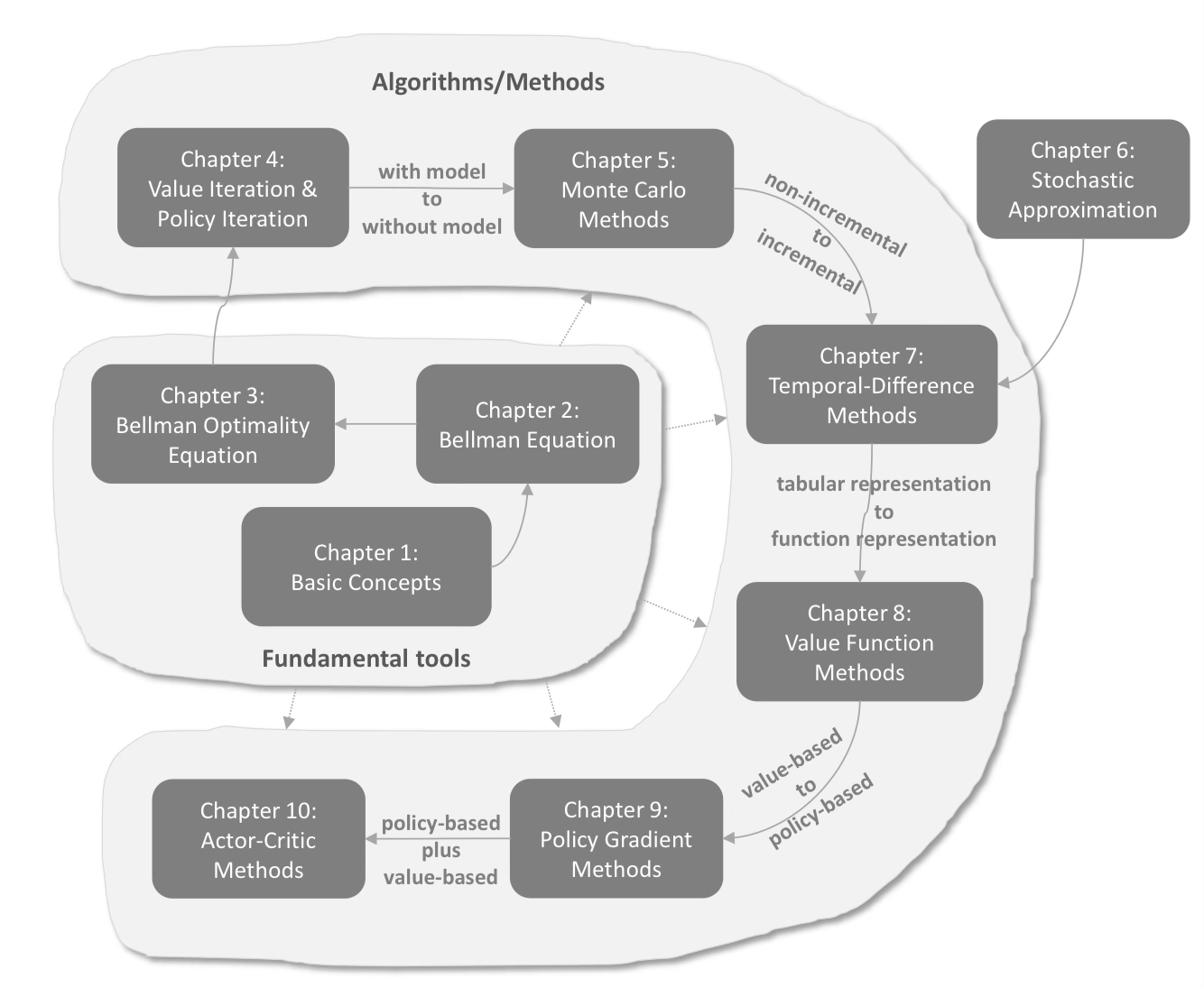
强化学习

基本概念

Eg. Grid

state
state space S
action
action space A(s)
State transition

• forbidden area
  Tabular representation: deterministic 因为事实上是三阶张量
  State transition probability: all situation
  Eg. p(s_2|s_1,a_2)

Policy
π(a_1|s_1)
Tabular representation: fit for all
实现：随机采样

Reward in R(s,a)
Eg. r_bound=-1,r_forbid=-1,r_target=1
table: deterministic
Mathematical: stochastic
Eg. p(r=1|s1,a1)
Hardworking->positive
Trajectories轨迹: a state-action-reward chain
Return of .:sum of reward. use to compare policy
Discount rate γ:balance future ,prevent cycle收敛

Episode :usually finite, have terminal->episodic
Continuing:
Episodic-> continuing: absorbing state or normal state with γ

MDP( Markov decision process )

• sets
  • S
  • A(s)
  • R(s, a)
• Probability distribution
  • State transition probability $p(v_f|v_i,a_k)$
  • Reward probability $p(r|v_f,a_k)$已考虑末状态和操作，不考虑初状态
• Policy
  • π(a|s)也是一种概率
• Markov property与之前的状态无关
  When decision is given ->Markov process

Bellman equation

State value: $v_\pi(s)=\mathbb E[G_t|S_t=s]$
Bootstrapping
矩阵形式$v_\pi=r_\pi+\gamma P_\pi v_\pi$
展开形式
$$
v_\pi(s)=\sum_a \pi(a|s)\sum _r p(r|s,a) r+\gamma\sum_a \pi(a|s) \sum_{s’} p(s’|s,a)v_\pi(s’)=\sum_a \pi(a|s)(\sum _r p(r|s,a) r+\gamma\sum_{s’} p(s’|s,a)v_\pi(s’))
$$
$S_t\xrightarrow{A_t}R_{t+1},S_{t+1}$ random variables
G_t: return of certain trajectory
convergence：Cauchy

随机变量$X|Y,Z\rightarrow p^x_{yz}$，YZ为伪指标，缩并$value^{x}_{yz}$得到期望$\mathbb E_{yz}$
分上下指标或用|或；分隔，从右往左，相同则不缩并，不同则所并~numpy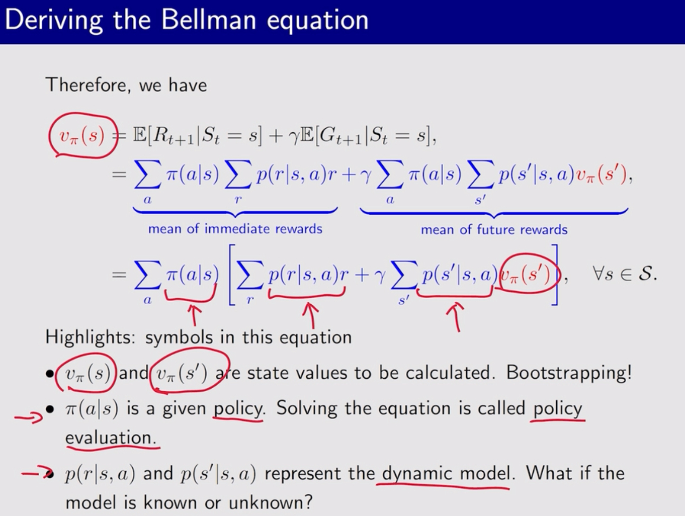

求解Closed-form solution $v=(1-\gamma P)^{-1}r$

• iterative solution 收敛

• action value $q(s, a) := \mathbb{E} \left[ R_t \mid S_t = s, A_t = a \right]$
  table: all situation
  $$
  v_\pi (s)=\sum_a \pi(a|s)q_\pi(s,a)
  $$
  $$
  q_\pi(s,a)=\sum_r p(r|s,a)r+\gamma \sum _{s’}p(s’|s,a)v_\pi(s’)
  $$
  不只考虑当前策略的

Bellman optimal equation (BOE)
$$
v(s)=\max_\pi(\sum_a \pi(a|s)\sum _r p(r|s,a) r+\gamma\sum_a \pi(a|s) \sum_{s’} p(s’|s,a)v_\pi(s’))=\max_a \pi(a|s)(\sum _r p(r|s,a) r+\gamma\sum_{s’} p(s’|s,a)v_\pi(s’))
$$
矩阵形式$v_\pi=\max _\pi(r_\pi +\gamma P_\pi v)$
注意括号里面向量v，理论上每个分量是关于π的函数，这里是对π取最值，使每个分量最大。而不是求无穷范数，也并没有引入模长
计算时可能不知道v(s’)需要值迭代等方法
分量是$\pi^a_s c_{sa}$ 固定s，只需找a使$c_{sa}$最大

• how: value iteration
  • policy update:先求最大π=argmax … 即最大值对的自变量的值（arguments of the maximum）
  • value update:再求v（s）(*)
• Contraction mapping theorem$||f(v_1)-f(v_2)||_\infty\leq \gamma ||v_1-v_2||_\infty$
  • existence
  • uniqueness
  • algorithm: exponential
• deterministic, greedy只选最大的
  • γ 减小，短视
  • 惩罚 增加
    • r->ar+b不变
  • 其实越晚到达奖励越少，所以不会扰远路

value iteration &policy iteration

dynamic programming, Model Based RL

policy iteration

• policy evaluation$v_{\pi _k}=r_{\pi _k} +\gamma P_{\pi _k} v_{\pi _k}$
  • iterative solution(*)直到误差足够小
• policy improvement$v_{\pi _{k+1}}=\text{argmax} _{\pi }(r_{\pi _k} +\gamma P_{\pi} v_{\pi _k})$
  • $v_{\pi _{k+1}}$>$v_{\pi _{k}}$
  • converges to an optimal policy
• 接近目标的先训练好

Truncated(截断) policy iteration algorithm
(*)步只进行j次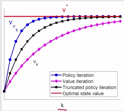

GPI: generalized policy iteration

Monto Carlo Learning

Without model, we need data!

model-free没有p的值，依赖数据(experience)
mean estimation
Law of Large number: $\mathbb E =\mathbb E [ x]$,$Var[\bar X]=\frac 1N{Var}{[X]}$

采样方法

MC basic

• policy evaluation:采样估计q
  • episode length
• policy improvement:

MC Exploring Starts
visit::state-action pair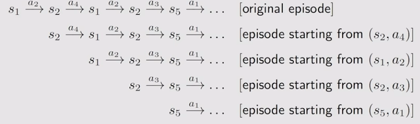

• first visit
• very visit
  从后往前
  Exploring：遍历
  Starts：从每个（s，a）开始

MC ε-Greedy
ε=0最优,逐渐减小
soft policy: stochastic
without Exploring Starts
$$

\pi(a|s) = \begin{cases} 1 - \frac{\epsilon}{|\mathcal{A}|}({|\mathcal{A}|}-1) & \text{if } a = \text{argmax}_a Q(s, a) \ \frac{\epsilon}{|\mathcal{A}|} & \text{if } a \neq \text{argmax}_a Q(s, a) \end{cases}

$$

• 拿出ε均分，剩下的给greedy
  exploitation& exploration~[[练习|展示区&学习区]]
  π在大π-ε中找，every visit

Stochastic Approximation

incremental
eg. $\bar x$增量式估计$w_{k+1}=w_{k}-a_k(w_{k}-x_{k})$ $a_k=\frac 1n$
$\Delta x = -ae(x)$~梯度下降，负反馈，a：步长

• 鞅论（Martingales）与随机逼近（Stochastic approximation） 保证了随机过程的收敛性

Robbins-Monro algorithm
$g(w)=0$ 不知道g
$w_{k+1}=w_k-a_k\tilde g(w_k,\eta _k)$ $\eta _k$噪声
$\lim w_k=w^*$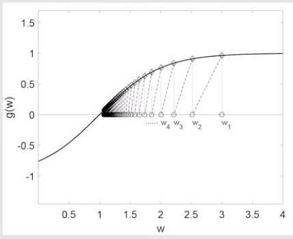

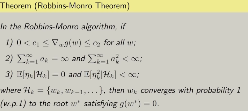
w.p.1: with probability 1=almost surely~测度论XI.1 几乎处处 Almost Everywhere - Skye的文章 - 知乎

1. 递增,有界
   • g=∇L 找的是损失函数
2. 收敛于0,但不太快
   • w_1不影响
   • eg. 1/k, sufficiently small number
3. eg. iid. independent and identically distributed

In general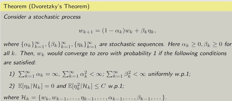

• 允许$\beta$很快收敛到0
• 运用伪鞅：期望不变
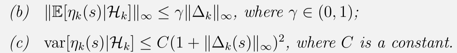
• 证明RM：运用中值定理$\Delta g(w)=\Delta w \cdot g’(w)$
• multiple variables:

Stochastic gradient descent

eg. mean estimation
优化$\min_w J(w)=\mathbb E[f(w,X)]$

gradient decent(GD)
let $\nabla_w \mathbb E[f(w,X)]=0$
$$
w_{k+1}=w_k-a_k\nabla_w \mathbb E[f(w_k,X)]=w_k-a_k \mathbb E[\nabla_wf(w_k,X)]=0
$$

batch gradient decent(BGD)
$\mathbb E[\nabla_wf(w,X)]\approx \frac 1n…$

• 函数需要在模型训练之前定义

Stochastic gradient decent(SGD)
$w_{k+1}=w_k-a_k\nabla_w f(w_k,x_k)$
n=1
convergence

• SGD is a special RM algorithm
• 较远时收敛较快
  
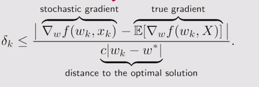
  deterministic->随机抽取

mini batch gradient decent(MBGD)
m=n时由于随机抽取，任有可能不是全部的

Temporal-Difference Learning

incremental, online, bootstrapping, low estimation variance, bias<->MC无偏估计
$$
q_{t+1}(s_t,a_t)=q_{t}(s_t,a_t)-\alpha_t(s_t,a_t)[q_{t}(s_t,a_t)-(r_{t+1}+\gamma \bar q_t)]
$$

$$
\underbrace{v_{t+1}\left(s_{t}\right)}_{\text {new estimate }}=\underbrace{v_{t}\left(s_{t}\right)}_{\text {current estimate }}-\alpha_{t}\left(s_{t}\right)[\overbrace{v_{t}\left(s_{t}\right)-(\underbrace{r_{t+1}+\gamma v_{t}\left(s_{t+1}\right)}_{\text {TD target } \bar{v}_{t}})}^{\text {TD error } \delta_{t}}]
$$
change form: $v_{t+1}\left(s_{t}\right)-\bar{v}_{t}=\left[1-\alpha_{t}\left(s_{t}\right)\right]\left[v_{t}\left(s_{t}\right)-\bar{v}_{t}\right]$, so it is called Temporal-Difference

Bellman expectation equation
RM算法中其实函数是未知的，用$v_k(s_k’)$代替$v_\pi(s_k’)$
收敛性：由于$v_t(s)$收敛于最大值，故$v_{t+1}(s)-v_t(s)$收敛于0且（sup，理解为带有噪声的）单调

Sarsa

Sarsa:$(s_t,a_t,r_{t+1},s_{t+1},a_{t+1})$
$$
q_{t+1}(s_t,a_t)=q_{t}(s_t,a_t)-\alpha_t(s_t,a_t)[q_{t}(s_t,a_t)-(r_{t+1}+\gamma q_t(s_{t+1},a_{t+1}))]
$$

• 这里的a_t+1是根据policy选的
• policy evaluation
• policy update
  • ε-greedy
• 特定目标可以只训练部分visit

Expected Sarsa
$$
q_{t+1}(s_t,a_t)=q_{t}(s_t,a_t)-\alpha_t(s_t,a_t)[q_{t}(s_t,a_t)-(r_{t+1}+\gamma \mathbb E [q_t(s_{t+1},A)])]
$$

• 综合考虑所有a_t+1

n-step Sarsa
$$
q_{t+1}(s_t,a_t)=q_{t}(s_t,a_t)-\alpha_t(s_t,a_t)[q_{t}(s_t,a_t)-\sum_{i=1}^nr ^{i-1}+\gamma^nq_t(s_{t+n},a_{t+n})]
$$

• 综合MC
• 综合variance &bias

Q-learning

use $\pi _b$ (behavior policy)to generate episode${s_0,a_0,r_1,s_1,a_1…}$
for each step:
update q-value
$$
q_{t+1}(s_t,a_t)=q_{t}(s_t,a_t)-\alpha_t(s_t,a_t)[q_{t}(s_t,a_t)-(r_{t+1}+\gamma \max _{a \in A }q_t(s_{t+1},a))]
$$
update policy $\pi_{T,t+1}$

• estimate optimal q
• update do not need π: off-policy
  • behavior policy
  • target policy
  • on-policy: behavior policy=target policy
  • off-policy: behavior policy, target policy can be difference ~ exploitation& exploration
• do not need ε-greedy: $\pi_b$ already have exploration

function approximation

v

input: table(discrete) ->function(continues)

• storage
• generalization ability

estimate:$\hat v (s,w)=\phi ^T(s)w$

• w: parameter vector
  • We can add dimension to increase accuracy
  • we did not use it before because the correspondence rule before is natural
• $\phi (s)$: feature vector of s.
• train to change w
• linear function was widely used before. then $\phi (s)$ can be polynomial basis, Fourier basis.
  • difficult to select
  • easy to analysis
  • can uniform tabular representation $\phi (s_i)=e_i,\nabla _w\hat v(s_i,w)=e_i$
• neural network are widely used nowadays

objective function(true value error)
$J(w)=\mathbb E[v_\pi(S)-\hat v (S,w)]^2$

• goal: minimize J(w)

• probability distribution of S

  • uniform, but some states are more important
  • stationary, long-run behavior $d_\pi(s)$
    • $d_\pi^T=d_\pi^T P_\pi$ eigenvalue

• Bellman error

• Projected Bellman error: 投到span$\phi (s)$

Sarsa:
$$
w_{t+1}=w_{t}+\alpha_{t}\left[r_{t+1}+\gamma \hat{q}\left(s_{t+1}, a_{t+1}, w_{t}\right)-\hat{q}\left(s_{t}, a_{t}, w_{t}\right)\right] \nabla_{w} \hat{q}\left(s_{t}, a_{t}, w_{t}\right)
$$
与table比多了$\nabla_{w} \hat{q}\left(s_{t}, a_{t}, w_{t}\right)$
Q-learning
$$
w_{t+1}=w_{t}+\alpha_{t}\left[r_{t+1}+\gamma \max _{a\in A} \hat{q}\left(s_{t+1}, a, w_{t}\right)-\hat{q}\left(s_{t}, a_{t}, w_{t}\right)\right] \nabla_{w} \hat{q}\left(s_{t}, a_{t}, w_{t}\right)
$$

Deep Q-learning(DQN)

network: function

• main network
• target network: fixed for some time and copy main
  $$
  J=\mathbb{E}\left[\left(R+\gamma \max _{a \in \mathcal{A}\left(S^{\prime}\right)} \hat{q}\left(S^{\prime}, a, w_{T}\right)-\hat{q}(S, A, w)\right)^{2}\right]
  $$

experience replay
replay buffer（缓冲区）$\mathcal{B} :=\left{\left(s, a, r, s^{\prime}\right)\right}$
use a mini-batch randomly from B
(S,A)is seemed as index, which assume to be i.i.d. , and we can use it for times, so we collect it and replay. In tabular cases, (S,A) is naturally independent.
$s\to W\to\hat q(s,a_i)$

π

Since s has been continuous, pi must use function to approach.
generate policy greedily from value ->train policy, use metrics(度规) to judge policy.

average state value：
$$
\bar{v}_{\pi}:=\mathbb{E}\left[v_{\pi}(S)\right]=d_sv^s_\pi=\mathbb{E}\left[\sum_{t=0}^{\infty} \gamma^{t} R_{t+1}\right]
$$

• d independent to pi, denote as $d_0,\bar v_\pi^0$
  • when interested in v_i, let d=e_i
• d dependent on pi: stationary

average reward
$$
\bar{r}_{\pi} := \sum_{s \in \mathcal{S}} d_{\pi}(s) r_{\pi}(s)=\mathbb{E}\left[r_{\pi}(S)\right]=\lim _{n \rightarrow \infty} \frac{1}{n} \mathbb{E}\left[\sum_{k=1}^{n} R_{t+k}\right]
$$

• can be undiscounted
• $\bar v_\pi=\bar r_\pi +\gamma \bar v_\pi$

$$
\nabla_{\theta} J(\theta)=\sum_{s \in \mathcal{S}} \eta(s) \sum_{a \in \mathcal{A}} \nabla_{\theta} \pi(a \mid s, \theta) q_{\pi}(s, a)
$$
use dx=x ln x , we get$=\mathbb{E}\left[\nabla_{\theta} \ln \pi(A \mid S, \theta) q_{\pi}(S, A)\right]$
to fit ln, we use softmax:
$$
\pi(a \mid s, \theta)=\frac{e^{\phi(s, a, \theta)}}{\sum_{a^{\prime} \in \mathcal{A}} e^{\phi\left(s, a^{\prime}, \theta\right)}}
$$
a neural network can help you do this automatically

• stochastic & exploratory

since $q_\pi$ is unknown
we can use MC (REINFORCE)
on policy
change form: $\theta_{t+1}=\theta_{t}+\alpha \underbrace{\left(\frac{q_{t}\left(s_{t}, a_{t}\right)}{\pi\left(a_{t} \mid s_{t}, \theta_{t}\right)}\right)}_{\beta_{t}} \nabla_{\theta} \pi\left(a_{t} \mid s_{t}, \theta_{t}\right)$ , which maximized (polarize, because the optimistic policy is deterministic) pi, balance exploitation & exploration

Actor-Critic

actor: update policy to act
critic: estimate policy to value

QAC

use TD to estimate $q_\pi$
(calculate q-error and update q_t)

A2C(advanced AC)

baseline
$$
b^{*}(s)=\frac{\mathbb{E}_{A \sim \pi}\left[\left|\nabla_{\theta} \ln \pi\left(A \mid s, \theta_{t}\right)\right|^{2} q(s, A)\right]}{\mathbb{E}_{A \sim \pi}\left[\left|\nabla_{\theta} \ln \pi\left(A \mid s, \theta_{t}\right)\right|^{2}\right]}\approx v_\pi (s)
$$

• does not change E, change Var
  advanced function(Zero-centered): $\delta_{\pi} := q_{\pi}(S, A)-v_{\pi}(S)\approx r_{t+1}+\gamma v_t(s_{t+1})-v_t(s_t)$, (have the same expectation ) which is TD error
  then we use delta to update both w for v(critic) & θ for π(actor)

Off-policy AC

Off-policy

• 之前的delta 依赖于pi
• importance sample: 用分布p_1估计p_0
• importance weight: $\frac {p_0(x_i)}{p_1(x_i)}$
• In continuous case, we can know $p_0(x_i)$, but we don not know $\mathbb E(X)=\int p_0(x) dx$
• value update can be off-policy as before : 不涉及状态的更新
• $\beta$ can be $\mu$+noise

Deterministic AC (DAC)

之前用了soft max，不是真实的连续输出
实际上输出的也只是每个值的概率
$a^._s=\mu (s;\theta)$ is deterministic ,实际上代替了$\pi^a_s$,本质上都是输入s输出a

$$
J(\theta)=\mathbb{E}\left[v_{\mu}(s)\right]=\sum_{s \in \mathcal{S}} d(s) v_{\mu}(s)
$$

• d independent to pi, denote as $d_0$
  • when interested in v_i, let d=e_i
    $$
    \nabla_{\theta} J(\theta)=\sum_{s \in \mathcal{S}} \rho_{\mu}(s) \nabla_{\theta} \mu(s)\left(\nabla_{\mu (s)} q_{\mu}(s, \mu(s))\right)
    $$

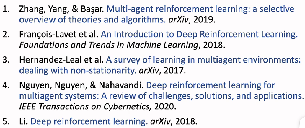
MARL

Multi-Agent Reinforcement Learning

【多智能体强化学习(1-2)：基本概念 Multi-Agent Reinforcement Learning】

• fully cooperative setting
• fully competitive setting
• Mixed cooperative & cooperative
• Self -Interested

$A^i_t,R^i_t,S_t,U^i_t ~~return,\pi (a^i|s;\theta ^i)$
$V_i(s_t;\theta ^1…\theta ^n)=\mathbb E[U^i_t|S_t=s_t]$ depend on all theta

convergence收敛:无法让收益更高
Nash equilibrium: While all the other agents’ policy remain the same, certain agent remains the same.
互相影响

• partial observation: $o^i$ 第i个的观测

• full observation

• fully decentralized

  • 不收敛

• fully centralized:

  • Actor-Critic method: $\pi(a^i|\mathbf o;\theta^i),q(\mathbf o,\mathbf a;w^i)$
  • slow

• Centralized training with decentralized execution

  • $\pi(a^i| o^i;\theta^i),q(\mathbf o,\mathbf a;w^i)$
    
    
    Parameter Sharing: 功能相同

HRL

• tensorflow的研究
• 一个足球模拟11v11但是c++
• 自动驾驶相关
• https://github.com/ray-project/ray/blob/master/rllib/examples/hierarchical/hierarchical_training.py
  但我发现很多地方看不懂，我可能需要先补一下前面的内容